catalyst.draw_graph
- draw_graph(qnode: QJIT, *, level: int | None = None) Callable[source]
Visualize a single QJIT compiled QNode, showing wire flow through quantum operations, program structure, and pass-by-pass impacts on compiled programs.
Note
The
draw_graphfunction visualizes a QJIT-compiled QNode in a similar manner as view-op-graph does in MLIR, which leverages Graphviz to show data-flow in the compiled IR.As such, use of
draw_graphrequires installation of Graphviz, pydot, and matplotlib software packages. Please consult the links provided for installation instructions.Additionally, it is recommended to use
draw_graphwith PennyLane’s program capture enabled (seeqp.capture.enable).Warning
This function only visualizes quantum operations contained in workflows involving a single
qjit-compiled QNode. Workflows involving multiple QNodes or operations outside QNodes cannot yet be visualized.Only transformations found within the Catalyst compiler can be visualized. Any PennyLane tape transform will have already been applied before lowering to MLIR and will appear as the base state (
level=0) in this visualization.Lastly,
catalyst.draw_graphis currently not compatible with dynamic wire allocation. This includespennylane.allocation.allocate()and dynamic wire allocation that may occur in MLIR directly (viaquantum.alloc_qbinstructions).- Parameters:
qnode (QJIT) – The input qjit-compiled QNode that is to be visualized. The QNode is assumed to be compiled with qjit.
level (int | None) – The level of transformation to visualize. If
None, the final level is visualized.
- Returns:
A function that has the same argument signature as the compiled QNode. When called, the function will return the graph as a tuple of (
matplotlib.figure.Figure,matplotlib.axes._axes.Axes) pairs.- Return type:
Callable
- Raises:
VisualizationError – If the circuit contains operations that cannot be converted to a graphical representation.
TypeError – If the
levelargument is not of type integer orNone. If the inputQNodeis not qjit-compiled.ValueError – If the
levelargument is a negative integer.
- Warns:
UserWarning – If the
levelargument provided is larger than the number of passes present in the compilation pipeline.
Example
Using
draw_graphrequires aqjit’d QNode and alevelargument, which denotes the cumulative set of applied compilation transforms (in the order they appear) to be applied and visualized.import pennylane as qp import catalyst qp.capture.enable() @qp.qjit @qp.transforms.merge_rotations @qp.transforms.cancel_inverses @qp.qnode(qp.device("null.qubit", wires=3)) def circuit(): qp.H(0) qp.T(1) qp.H(0) qp.RX(0.1, wires=0) qp.RX(0.2, wires=0) return qp.expval(qp.X(0))
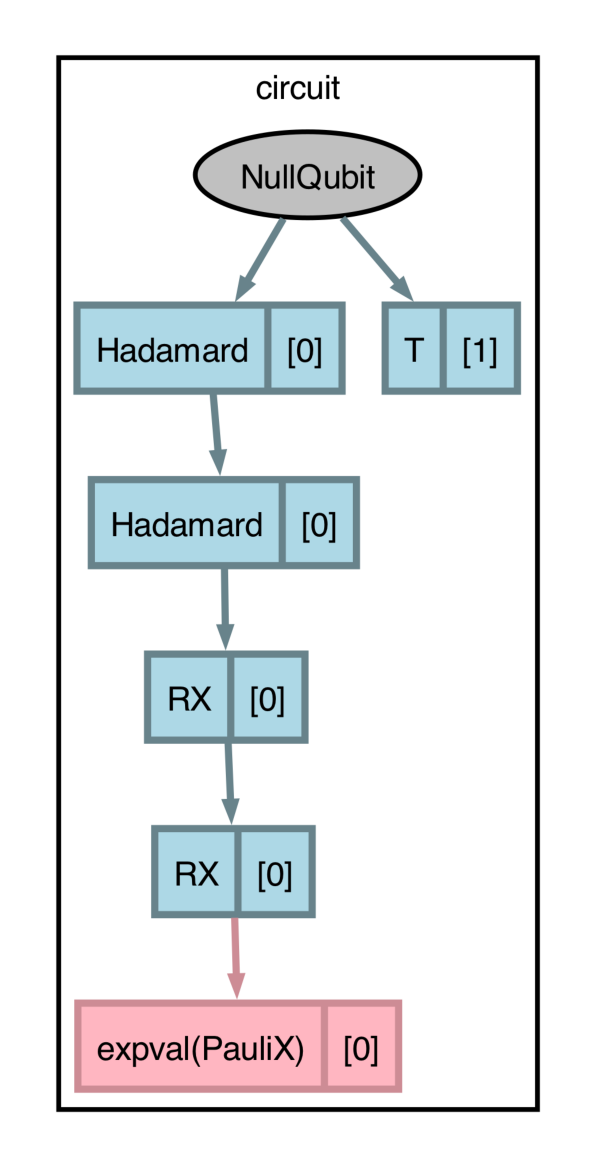
With
level=0, the graphical visualization will display the program as if no transforms are applied:>>> fig, ax = catalyst.draw_graph(circuit, level=0)() >>> fig.savefig('path_to_file.png', dpi=300, bbox_inches="tight")
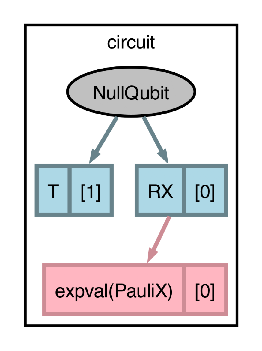
Though you can
printthe output ofcatalyst.draw_graph, it is recommended to use thesavefigmethod ofmatplotlib.figure.Figurefor better control over image resolution (DPI). Please consult the matplotlib documentation for usage details ofsavefig.With
level=2, bothmerge_rotations()andcancel_inverses()will be applied, resulting in the two Hadamards cancelling and the two rotations merging:>>> fig, ax = catalyst.draw_graph(circuit, level=2)() >>> fig.savefig('path_to_file.png', dpi=300, bbox_inches="tight")
Usage Details
Visualizing Control Flow
The
draw_graphfunction can be used to visualize control flow, resulting in a scalable representation that preserves program structure:@qp.qjit(autograph=True) @qp.qnode(qp.device("null.qubit", wires=3)) def circuit(): qp.H(0) for i in range(3): if i == 1: qp.X(0) elif i == 2: qp.Y(0) else: qp.Z(0) return qp.probs()
>>> fig, ax = catalyst.draw_graph(circuit)()
>>> fig.savefig('path_to_file.png', dpi=300, bbox_inches="tight")
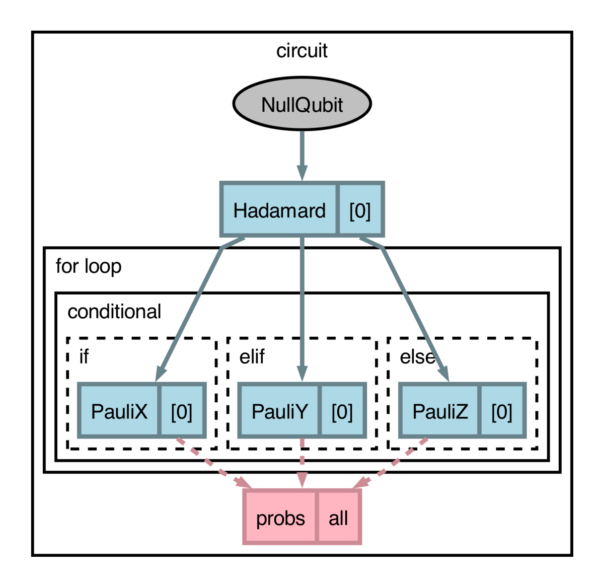
As one can see, the program structure is preserved in the figure.
Visualizing Dynamic Circuits
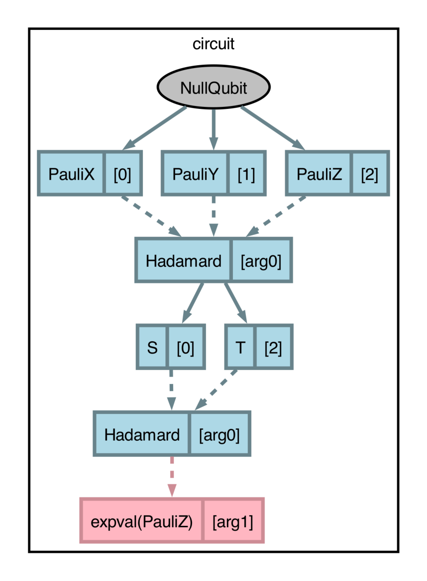
Circuits can depend on parameters that are not known at compile time, which result in conventional visualization tools failing. Consider the following circuit.
@qp.qjit
@qp.qnode(qp.device("null.qubit", wires=3))
def circuit(x, y):
    qp.X(0)
    qp.Y(1)
    qp.Z(2)
    qp.H(x) # 'x' is a dynamic wire index
    qp.S(0)
    qp.T(2)
    qp.H(x)
    return qp.expval(qp.Z(y))
The two
qp.Hgates act on wires that are dynamic. In order to preserve qubit data flow, each dynamic operator acts as a “choke point” to all currently active wires. To visualize this clearly, we use dashed lines to represent a dynamic dependency and solid lines for static/known values:>>> x, y = 1, 0 >>> fig, ax = catalyst.draw_graph(circuit)(x, y) >>> fig.savefig('path_to_file.png', dpi=300, bbox_inches="tight")