%pip install jaxopt

Qubit Rotation

Note

This tutorial is a Catalyst adaptation of the Pennylane Qubit Rotation tutorial by Josh Izaac.

To see how to use Catalyst with PennyLane, let’s consider the ‘hello world’ program of quantum machine learning (QML):

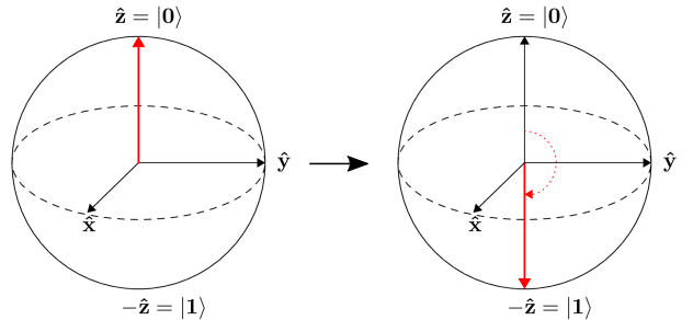
The task at hand is to optimize the angle parameters of two rotation gates in order to flip a single qubit from state \(\left|0\right\rangle\) to state \(\left|1\right\rangle\).

The quantum circuit

In the qubit rotation example, we wish to implement the following quantum circuit:

Breaking this down step-by-step, we first start with a qubit in the ground state \(|0\rangle = \begin{bmatrix}1 & 0 \end{bmatrix}^T\), and rotate it around the x-axis by applying the gate

\[\begin{split}\begin{aligned} R_x(\phi_1) = e^{-i \phi_1 \sigma_x /2} = \begin{bmatrix} \cos \frac{\phi_1}{2} & -i \sin \frac{\phi_1}{2} \\ -i \sin \frac{\phi_1}{2} & \cos \frac{\phi_1}{2} \end{bmatrix}, \end{aligned}\end{split}\]

and then around the y-axis via the gate

\[\begin{split}\begin{aligned} R_y(\phi_2) = e^{-i \phi_2 \sigma_y/2} = \begin{bmatrix} \cos \frac{\phi_2}{2} & - \sin \frac{\phi_2}{2} \\ \sin \frac{\phi_2}{2} & \cos \frac{\phi_2}{2} \end{bmatrix}. \end{aligned}\end{split}\]

After these operations the qubit is now in the state

\[| \psi \rangle = R_y(\phi_2) R_x(\phi_1) | 0 \rangle.\]

Finally, we measure the expectation value \(\langle \psi \mid \sigma_z \mid \psi \rangle\) of the Pauli-Z operator

\[\begin{split}\begin{aligned} \sigma_z = \begin{bmatrix} 1 & 0 \\ 0 & -1 \end{bmatrix}. \end{aligned}\end{split}\]

Using the above to calculate the exact expectation value, we find that

\[\langle \psi \mid \sigma_z \mid \psi \rangle = \langle 0 \mid R_x(\phi_1)^\dagger R_y(\phi_2)^\dagger \sigma_z R_y(\phi_2) R_x(\phi_1) \mid 0 \rangle = \cos(\phi_1)\cos(\phi_2).\]

Depending on the circuit parameters \(\phi_1\) and \(\phi_2\), the output expectation lies between \(1\) (if \(\left|\psi\right\rangle = \left|0\right\rangle\)) and \(-1\) (if \(\left|\psi\right\rangle = \left|1\right\rangle\)).

Let’s see how we can easily implement and optimize this circuit using PennyLane.

Importing PennyLane and Catalyst

In order to use PannyLane with the Catalyst compiler, we need to import several important components:

• The PennyLane framework in order to access the base QML API,

• The Catalyst Python package,

• The JAX version of NumPy.

import pennylane as qml
from catalyst import qjit, grad
import jax.numpy as jnp

Creating a device

Before we can construct our quantum node, we need to initialize a PennyLane device.

Definition

Any computational object that can apply quantum operations and return a measurement valueis called a quantum device.

In PennyLane, a device could be a hardware device (such as the IBM QX4, via the PennyLane-PQ plugin), or a software simulator (such as Strawberry Fields, via the PennyLane-SF plugin).

Catalyst supports a subset of devices available in PennyLane. For this tutorial, we are using the qubit model, so let’s initialize the lightning.qubit device provided by PennyLane for the PennyLane-Lightning simulator.

dev1 = qml.device("lightning.qubit", wires=1)

Preparing the compiled quantum function

Now that we have initialized our device, we can begin to construct a Quantum circuit.

First, we need to define the quantum function that will be evaluated in the circuit:

def circuit(params):
    qml.RX(params[0], wires=0)
    qml.RY(params[1], wires=0)
    return qml.expval(qml.PauliZ(0))

This is a simple circuit, matching the one described above. Notice that the function circuit() is constructed as if it were any other Python function; it accepts a positional argument params, which may be a list, tuple, or array, and uses the individual elements for gate parameters.

However, quantum functions are a restricted subset of Python functions. For a Python function to also be a valid quantum function, there are some important restrictions:

• Quantum functions must contain quantum operations, one operation per line, in the order in which they are to be applied. In addition, we must always specify the subsystem the operation applies to, by passing the wires argument; this may be a list or an integer, depending on how many wires the operation acts on.

• Quantum functions must return either a single or a tuple of measured observables. In Catalyst, quantum functions may also return values of JAX types representing classical data. As a result, the quantum function always returns a classical quantity, allowing the QNode to interface with other classical functions (and also other QNodes).

Certain devices may only support a subset of the available PennyLane operations/observables, or may even provide additional operations/observables. Please consult the documentation for the plugin/device for more details.

Once we have written the quantum function, we convert it into a pennylane.QNode running on device dev1 by applying the pennylane.qnode decorator directly above the function definition:

@qml.qnode(device=dev1)
def circuit(params):
    qml.RX(params[0], wires=0)
    qml.RY(params[1], wires=0)
    return qml.expval(qml.PauliZ(0))

Thus, our circuit() quantum function is now a quantum function, which will become the subject of certain quantum-specific optimisations and then run on our device every time it is evaluated. Catalyst supports compiling such functions and, as we will see later, it also allows us to compile their derivatives.

To compile the quantum circuit function, we must trace it first with JAX, by defining a JAX entry point annotated with the qjit decorator. In addition to the functionality usually provided by the standard jax.jit function, qjit is aware of quantum-specific compilation techniques. In this tutorial we always define JAX entry points as a separate Python functions which have jit_ prefix in their names.

@qjit
def jit_circuit(params):
    return circuit(params)

print(jit_circuit(jnp.array([0.54, 0.12])))

0.8515405859048367

We can always use qjit as a funciton rather as a decorator. When used this way, qjit accepts a function to compile and returns a callable Python object. In order to call the compiled function, we must call the object by passing it the required parameters as we did previously.

jit_circuit = qjit(circuit)
print(jit_circuit(jnp.array([0.54, 0.12])))

0.8515405859048367

Compiling quantum gradients

The gradient of the function circuit, can be evaluated by utilizing the same compilation pipeline that we used to evaluate the function itself.

PennyLane and Catalyst incorporate both analytic differentiation, as well as numerical methods (such as the method of finite differences). Both of these are done without the need for manual programming of the derivatives.

We can differentiate quantum functions inside the QJIT context by using the grad function provided by Catalyst. This function operates on a QNode and returns another function representing its gradient (i.e., the vector of partial derivatives).

By default, grad will compute the derivate with respect to the first function argument, but any (one or more) argument can be specified via the argnum keyword argument. In this case, the function circuit takes one argument (params), so we specify argnum=0. Because the argument has two elements, the returned gradient is two-dimensional. In order to test our gradient function, we compile it with qjit.

jit_dcircuit = qjit(grad(circuit, argnum=0))
print(jit_dcircuit(jnp.array([0.54, 0.12])))

[-0.51043869 -0.10267824]

A note on arguments

Quantum circuit functions, being a restricted subset of Python functions, can also make use of multiple positional arguments and keyword arguments. For example, we could have defined the above quantum circuit function using two positional arguments, instead of one array argument:

@qml.qnode(device=dev1)
def circuit2(phi1, phi2):
    qml.RX(phi1, wires=0)
    qml.RY(phi2, wires=0)
    return qml.expval(qml.PauliZ(0))

When we calculate the gradient for such a function, the usage of argnum will be slightly different. In this case, argnum=0 will return the gradient with respect to only the first parameter (phi1), and argnum=1 will give the gradient for phi2. To get the gradient with respect to both parameters, we can use argnum=[0,1]:

print(qjit(grad(circuit2, argnum=[0,1]))(0.54, 0.12))

[array(-0.51043869), array(-0.10267824)]

Compiling parts of the optimization loop

If using the default NumPy/Autograd interface, PennyLane provides a collection of optimizers based on gradient descent. These optimizers accept a cost function and initial parameters, and utilize PennyLane’s automatic differentiation to perform gradient descent.

Next, let’s make use of PennyLane’s built-in optimizers to optimize the two circuit parameters \(\phi_1\) and \(\phi_2\) such that the qubit, originally in state \(\left|0\right\rangle\), is rotated to be in state \(\left|1\right\rangle\). This is equivalent to measuring a Pauli-Z expectation value of \(-1\), since the state \(\left|1\right\rangle\) is an eigenvector of the Pauli-Z matrix with eigenvalue \(\lambda=-1\).

In other words, the optimization procedure will find the weights \(\phi_1\) and \(\phi_2\) that result in the following rotation on the Bloch sphere:

To do so, we need to define a cost and gradient functions. By minimizing the cost function, the optimizer will determine the values of the circuit parameters that produce the desired outcome.

In this case, our desired outcome is a Pauli-Z expectation value of \(-1\). Since we know that the Pauli-Z expectation is bound between \([-1, 1]\), we can define our cost directly as a JIT function. Another JIT function is required to calculate the gradient of our circuit.

# Optimization cost entry point
jit_cost = qjit(circuit)
# Optization gradient entry point
jit_grad = qjit(grad(circuit))

To begin our optimization, let’s choose small initial values of \(\phi_1\) and \(\phi_2\):

init_params = jnp.array([0.011, 0.012])
print(jit_cost(init_params))

0.9998675058299389

We can see that, for these initial parameter values, the cost function is close to \(1\).

# set the number of steps
steps = 100
# set the initial parameter values
params = init_params
# step of the gradient descend
stepsize = 0.4

for i in range(steps):
    # update the circuit parameters
    dp = jit_grad(params)
    params = params - stepsize*dp

    if (i + 1) % 5 == 0:
        print("Cost after step {:5d}: {: .7f}".format(i + 1, jit_cost(params)))

opt_1 = params
print("Optimized rotation angles: {}".format(opt_1))

Cost after step     5:  0.9961778
Cost after step    10:  0.8974935
Cost after step    15:  0.1440475
Cost after step    20: -0.1536720
Cost after step    25: -0.9152496
Cost after step    30: -0.9994046
Cost after step    35: -0.9999964
Cost after step    40: -1.0000000
Cost after step    45: -1.0000000
Cost after step    50: -1.0000000
Cost after step    55: -1.0000000
Cost after step    60: -1.0000000
Cost after step    65: -1.0000000
Cost after step    70: -1.0000000
Cost after step    75: -1.0000000
Cost after step    80: -1.0000000
Cost after step    85: -1.0000000
Cost after step    90: -1.0000000
Cost after step    95: -1.0000000
Cost after step   100: -1.0000000
Optimized rotation angles: [-4.9759957e-08  3.1415926e+00]

We can see that the optimization converges after approximately 40 steps.

Substituting this into the theoretical result \(\langle \psi \mid \sigma_z \mid \psi \rangle = \cos\phi_1\cos\phi_2\), we can verify that this is indeed one possible value of the circuit parameters that produces \(\langle \psi \mid \sigma_z \mid \psi \rangle=-1\), resulting in the qubit being rotated to the state \(\left|1\right\rangle\).

Compiling the whole optimization loop using JAX

We can easily combine the quantum parts of the program with the JAX code. Below we show how to implement the whole optimization loop in JAX. We make use of standard JAX control-flow primitives here.

from jax.lax import fori_loop

@qjit
def jit_opt(init_params):
    """ Compiled optimization loop function """
    stepsize = 0.4
    nsteps = 100

    def loop(i,p):
        dp = grad(circuit)(p)
        p2 = p - stepsize*dp
        return p2

    params = fori_loop(0, nsteps, loop, init_params)
    return params


opt_2 = jit_opt(jnp.array([0.011, 0.012]))
print(opt_2)

[-4.9759957e-08  3.1415926e+00]

Using third-party JAX libraries

We can combine our quantum functions with any Python libraries supporting JAX. In this section we use jaxopt.GradientDescent optimizer to solve the same optimization task.

from jaxopt import GradientDescent

@qjit
def jit_opt_thirdparty():

    def _target(x):
        p = jnp.array([x[0],x[1]])
        g = grad(circuit)(p)
        c = circuit(p)
        return c,(g[0],g[1])

    opt = GradientDescent(_target,
                          stepsize=0.4,
                          value_and_grad=True)

    steps = 100
    params = init_params[0],init_params[1]
    state = opt.init_state(params)

    def loop(i,arg):
        (p, s) = arg
        (p2, s2) = opt.update(p, s)
        return (p2, s2)

    (params, _) = fori_loop(0, steps, loop, (params,state))
    return jnp.array([params[0],params[1]])

opt_3 = jit_opt_thirdparty()
print(opt_3)

[-4.85367987e-08  3.14159261e+00]

Finally, we check that all the results obtained in this tutorial are consistant

assert jnp.allclose(opt_1, opt_2, atol=1e-7)
assert jnp.allclose(opt_1, opt_3, atol=1e-7)

doc/demos/qml/tutorial_qubit_rotation.ipynb

demos/qml/tutorial_qubit_rotation

 

Download Python script

 

Download Notebook

 

View on GitHub