qml.pulse.ParametrizedHamiltonian

class ParametrizedHamiltonian(coeffs, observables)

Bases: object

Callable object holding the information representing a parametrized Hamiltonian.

The Hamiltonian can be represented as a linear combination of other operators, e.g.,

\[H(\{v_j\}, t) = H_\text{drift} + \sum_j f_j(v_j, t) H_j\]

where the \(\{v_j\}\) are trainable parameters for each scalar-valued parametrization \(f_j\), and t is time.

Parameters

• coeffs (Union[float, callable]) – coefficients of the Hamiltonian expression, which may be constants or parametrized functions. All functions passed as coeffs must have two arguments, the first one being the trainable parameters and the second one being time.

• observables (Iterable[Operator]) – observables in the Hamiltonian expression, of same length as coeffs

A ParametrizedHamiltonian is a callable with the fixed signature H(params, t), with params being an iterable where each element corresponds to the parameters of each scalar-valued function of the Hamiltonian.

Calling the ParametrizedHamiltonian returns an Operator representing an instance of the Hamiltonian with the specified parameter values.

See also

evolve(), ParametrizedEvolution

Note

The ParametrizedHamiltonian must be Hermitian at all times. This is not explicitly checked; ensuring a correctly defined Hamiltonian is the responsibility of the user.

Example

A ParametrizedHamiltonian can be created using dot(), by passing a list of coefficients, as well as a list of corresponding observables. Each coefficient function must take two arguments, the first one being the trainable parameters and the second one being time, though it need not use them both.

f1 = lambda p, t: p[0] * jnp.sin(p[1] * t)
f2 = lambda p, t: p * t
coeffs = [2., f1, f2]
observables =  [qml.X(0), qml.Y(0), qml.Z(0)]
H = qml.dot(coeffs, observables)

The resulting object can be passed parameters, and will return an Operator representing the ParametrizedHamiltonian with the specified parameters. Note that parameters must be passed in the order the functions were passed in creating the ParametrizedHamiltonian:

p1 = jnp.array([1., 1.])
p2 = 1.
params = [p1, p2]  # p1 is passed to f1, and p2 to f2

>>> H(params, t=1.)
(
    2.0 * X(0)
  + 0.8414709848078965 * Y(0)
  + 1.0 * Z(0)
)

Note

To be able to compute the time evolution of the Hamiltonian with evolve(), these coefficient functions should be defined using jax.numpy rather than numpy.

We can also access the fixed and parametrized terms of the ParametrizedHamiltonian. The fixed term is an Operator, while the parametrized term must be initialized with concrete parameters to obtain an Operator:

>>> H.H_fixed()
2.0 * X(0)
>>> H.H_parametrized([[1.2, 2.3], 4.5], 0.5)
1.095316728312625 * Y(0) + 2.25 * Z(0)

Usage Details

An alternative method for creating a ParametrizedHamiltonian is to multiply operators and callable coefficients:

def f1(p, t):
    return jnp.sin(p[0] * t**2) + p[1]

def f2(p, t):
    return p * jnp.cos(t)

H = 2 * qml.X(0) + f1 * qml.Y(0) + f2 * qml.Z(0)

Note

Whichever method is used for initializing a ParametrizedHamiltonian, the terms defined with fixed coefficients should come before parametrized terms to prevent discrepancy in the wire order.

Note

The parameters used in the ParametrizedHamiltonian call should have the same order as the functions used to define this Hamiltonian. For example, we could call the above Hamiltonian using the following parameters:

>>> params = [[4.6, 2.3], 1.2]
>>> H(params, t=0.5)
(
    2 * X(0)
  + 3.212763940260521 * Y(0)
  + 1.0530990742684472 * Z(0)
)

Internally we are computing f1([4.6, 2.3], 0.5) and f2(1.2, 0.5).

Parametrized coefficients can be any callable that takes (p, t) and returns a scalar. It is not a requirement that both p and t be used in the callable: for example, the convenince function constant() takes (p, t) and returns p.

Warning

When initializing a ParametrizedHamiltonian via a list of parametrized coefficients, it is possible to create a list of multiple coefficients of the same form iteratively using lambda functions, i.e.

coeffs = [lambda p, t: p for _ in range(3)].

Do not, however, define the function as dependent on the value that is iterated over. That is, it is not possible to define

coeffs = [lambda p, t: p * t**i for i in range(3)]

to create a list

coeffs = [(lambda p, t: p), (lambda p, t: p * t), (lambda p, t: p * t**2)].

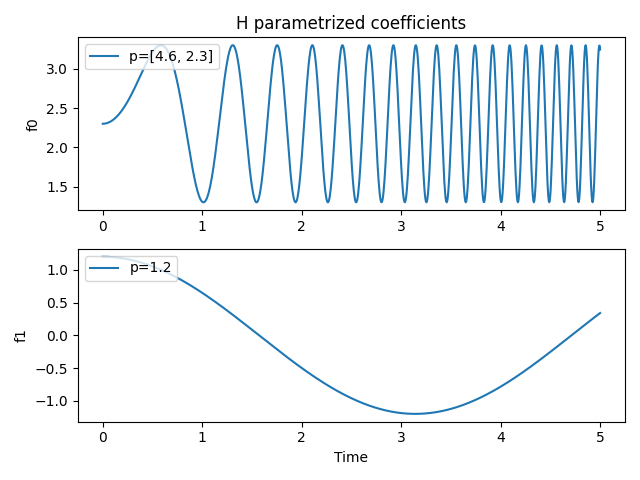
The value of i when creating the lambda functions is set to be the final value in the iteration, such that this will produce three identical functions

coeffs = [(lambda p, t: p * t**2)] * 3.

We can visualize the behaviour in time of the parametrized coefficients for a given set of parameters. Here we look at the Hamiltonian created above:

import matplotlib.pyplot as plt

times = jnp.linspace(0., 5., 1000)
fs = tuple(c for c in H.coeffs if callable(c))
params = [[4.6, 2.3], 1.2]

fig, axs = plt.subplots(nrows=len(fs))

for n, f in enumerate(fs):
    ax = axs[n]
    ax.plot(times, f(params[n], times), label=f"p={params[n]}")
    ax.set_ylabel(f"f{n}")
    ax.legend(loc="upper left")

ax.set_xlabel("Time")
axs[0].set_title(f"H parametrized coefficients")
plt.tight_layout()
plt.show()

It is possible to add two instance of ParametrizedHamiltonian together. The resulting ParametrizedHamiltonian takes a list of parameters that is a concatenation of the initial two Hamiltonian parameters:

coeffs = [lambda p, t: jnp.sin(p*t) for _ in range(2)]
ops = [qml.X(0), qml.Y(1)]
H1 = qml.dot(coeffs, ops)

def f1(p, t): return t + p
def f2(p, t): return p[0] * jnp.sin(p[1] * t**2)
H2 = f1 * qml.Y(0) + f2 * qml.X(1)

params1 = [2., 3.]
params2 = [4., [5., 6.]]

>>> H3 = H2 + H1
>>> H3([4., [5., 6.], 2., 3.], t=1)
(
    5.0 * Y(0)
  + -1.3970774909946293 * X(1)
  + 0.9092974268256817 * X(0)
  + 0.1411200080598672 * Y(1)
)

Attributes

coeffs	Return the coefficients defining the ParametrizedHamiltonian, including the unevaluated functions for the parametrized terms.
ops	Return the operators defining the ParametrizedHamiltonian.

coeffs

Return the coefficients defining the ParametrizedHamiltonian, including the unevaluated functions for the parametrized terms.

Returns

coefficients in the Hamiltonian expression

Return type

Iterable[float, Callable])

ops

Return the operators defining the ParametrizedHamiltonian.

Returns

observables in the Hamiltonian expression

Return type

Iterable[Operator]

Methods

H_fixed()	The fixed term(s) of the ParametrizedHamiltonian.
H_parametrized(params, t)	The parametrized terms of the Hamiltonian for the specified parameters and time.
map_wires(wire_map)	Returns a copy of the current ParametrizedHamiltonian with its wires changed according to the given wire map.

H_fixed()

The fixed term(s) of the ParametrizedHamiltonian. Returns a Sum operator of SProd operators (or a single SProd operator in the event that there is only one term in H_fixed).

H_parametrized(params, t)

The parametrized terms of the Hamiltonian for the specified parameters and time.

Parameters

• params (tensor_like) – the parameters values used to evaluate the operators

• t (float) – the time at which the operator is evaluated

Returns

a Sum of SProd operators (or a single SProd operator in the event that there is only one term in H_parametrized).

Return type

Operator

map_wires(wire_map)

Returns a copy of the current ParametrizedHamiltonian with its wires changed according to the given wire map.

Parameters

wire_map (dict) – dictionary containing the old wires as keys and the new wires as values

Returns

A new instance with mapped wires

Return type

ParametrizedHamiltonian

code/api/pennylane.pulse.ParametrizedHamiltonian

 

Download Python script

 

Download Notebook

 

View on GitHub