qml.fourier

Overview

This module contains functions to analyze the Fourier representation of quantum circuits.

Functions

circuit_spectrum(tape[, encoding_gates, ...])	Compute the frequency spectrum of the Fourier representation of simple quantum circuits ignoring classical preprocessing.
coefficients(f, n_inputs, degree[, ...])	Computes the first \(2d+1\) Fourier coefficients of a \(2\pi\) periodic function, where \(d\) is the highest desired frequency (the degree) of the Fourier spectrum.
get_spectrum(op, decimals)	Extract the frequencies contributed by an input-encoding gate to the overall Fourier representation of a quantum circuit.
join_spectra(spec1, spec2)	Join two sets of frequencies that belong to the same input.
qnode_spectrum(qnode[, encoding_args, ...])	Compute the frequency spectrum of the Fourier representation of quantum circuits, including classical preprocessing.
reconstruct(qnode[, ids, nums_frequency, ...])	Reconstruct an expectation value QNode along a single parameter direction.

Visualization

Tools to visualize the Fourier representations can be found in the fourier.visualize submodule. This requires the matplotlib package to be installed.

bar(coeffs, n_inputs, ax[, colour_dict, ...])	Plot a set of Fourier coefficients as a bar plot.
box(coeffs, n_inputs, ax[, colour_dict, ...])	Plot a list of sets of Fourier coefficients as a box plot.
panel(coeffs, n_inputs, ax[, colour])	Plot a list of sets of coefficients in the complex plane for a 1- or 2-dimensional function.
radial_box(coeffs, n_inputs, ax[, ...])	Plot a list of sets of Fourier coefficients on a radial plot as box plots.
violin(coeffs, n_inputs, ax[, colour_dict, ...])	Plots a list of sets of Fourier coefficients as a violin plot.

Fourier representation of quantum circuits

Consider a quantum circuit that depends on a parameter vector \(x\) with length \(N\). The circuit involves application of some unitary operations \(U(x)\), and then measurement of an observable \(\hat{O}\). Analytically, the expectation value is

\[\langle \hat{O} \rangle = \langle 0 \vert U^\dagger (x) \hat{O} U(x) \vert 0\rangle = \langle \psi(x) \vert \hat{O} \vert \psi (x)\rangle.\]

This output is simply a function \(f(x) = \langle \psi(x) \vert \hat{O} \vert \psi (x)\rangle\). Notably, it is a periodic function of the parameters, and it can thus be expressed as a multidimensional Fourier series:

\[f(x) = \sum \limits_{n_1\in \Omega_1} \dots \sum \limits_{n_N \in \Omega_N} c_{n_1,\dots, n_N} e^{-i x_1 n_1} \dots e^{-i x_N n_N},\]

where \(n_i\) are integer-valued frequencies, \(\Omega_i\) are the set of available values for the integer frequencies, and the \(c_{n_1,\ldots,n_N}\) are Fourier coefficients.

As a simple example, consider simple_circuit below, which is a function of a single parameter.

import pennylane as qml
from pennylane import numpy as np

dev = qml.device('default.qubit', wires=2)

@qml.qnode(dev)
def simple_circuit(x):
    qml.RX(x[0], wires=0)
    qml.RY(x[0], wires=1)
    qml.CNOT(wires=[1, 0])
    return qml.expval(qml.PauliZ(0))

We can mathematically evaluate the expectation value of this function to be \(\langle Z \rangle = 0.5 + 0.5 \cos(2x)\). Thus, the Fourier coefficients of this function are \(c_0 = 0.5\), \(c_1 = c^*_{-1} = 0\), and \(c_2 = c^*_{-2} = 0.25\).

The PennyLane fourier module enables calculation of the values of the Fourier coefficients \(c_{n_1,\dots, n_N}\). Knowledge of the coefficients, and thereby the spectrum of frequencies where the coefficients are non-zero, is important for the study of the expressivity of quantum circuits, as described in Schuld, Sweke and Meyer (2020) and Vidal and Theis, 2019 – the more coefficients available to a quantum model, the larger the class of functions that model can represent, potentially leading to greater utility for quantum machine learning applications.

Calculating the frequencies supported by a circuit

For certain circuits, information on the frequency spectra \(\Omega_j\) can be derived solely from the structure of the gates that encode the corresponding inputs \(x_j\) (see for example Schuld, Sweke, and Meyer (2020)). More precisely, if all input-encoding gates are of the form \(e^{-ix_j G}\), where \(G\) is a Hermitian operator that “generates” the operation, we can deduce a maximum set of frequencies that can theoretically appear in \(\Omega_j\). Depending on the non-input-encoding gates in the circuit, some of these theoretically supported frequencies may end up having vanishing Fourier coefficients, and \(\Omega_j\) effectively turns out to be smaller. However, estimates based on the input-encoding strategy can still be useful to understand the potential expressivity of a type of ansatz.

The theoretically supported frequencies can be computed using the circuit_spectrum() function. To mark which gates encode inputs (and, for example, which ones are only used for trainable parameters), we have to give input-encoding gates an id:

import pennylane as qml

dev = qml.device('default.qubit', wires=2)

@qml.qnode(dev)
def simple_circuit_marked(x):
    qml.RX(x[0], wires=0, id="x")
    qml.RY(x[0], wires=1, id="x")
    qml.CNOT(wires=[1, 0])
    return qml.expval(qml.PauliZ(0))

We can then compute the frequencies supported by the input-encoding gates as:

>>> from pennylane.fourier import circuit_spectrum
>>> freqs = circuit_spectrum(simple_circuit_marked)([0.1])
>>> for k, v in freqs.items():
>>>     print(k, ":", v)

x : [-2.0, -1.0, 0.0, 1.0, 2.0]

Note

Some encoding-gate types may give rise to non-integer-valued frequencies. In this case, the circuit_spectrum() function computes the frequency sets \(\Omega_j\) of the Fourier sum of the form

\[f(x) = \sum \limits_{\omega_1\in \Omega_1} \dots \sum \limits_{\omega_N \in \Omega_N} c_{\omega_1,\dots, \omega_N} e^{-i x_1 \omega_1} \dots e^{-i x_N \omega_N},\]

with \(\omega \in \mathbb{R}\). Just like any other function, such a sum can be turned into a proper Fourier series, but the mapping from non-integer-valued to integer-valued frequencies is not always trivial.

Calculating the Fourier coefficients

To get a more accurate picture of the Fourier series representation of a quantum circuit, we have to compute the Fourier coefficients \(c_{n_1,\ldots,n_N}\). This is done using numerical methods in the coefficients() function:

>>> from pennylane.fourier import coefficients
>>> coeffs = coefficients(simple_circuit, 1, 2)
>>> print(np.round(coeffs, decimals=4))
[0.5 +0.j 0.  -0.j 0.25+0.j 0.25+0.j 0.  -0.j]

The inputs to the coefficients() function are

• A function, or QNode containing the variational circuit for which to compute the Fourier coefficients,

• the length of the input vector, and

• the maximum frequency for which to calculate the coefficients (also known as the degree).

Internally, the coefficients are computed using NumPy’s discrete Fourier transform function. The order of the coefficients in the output thus follows the standard output ordering, i.e., \([c_0, c_1, c_2, c_{-2}, c_{-1}]\), and similarly for multiple dimensions. The normalization convention used here corresponds to the norm="forward" option in the NumPy transforms, i.e., the Fourier transform over an array of size \(N\) is rescaled by \(1/N\), while the inverse Fourier transform is left as-is.

For more details and examples of coefficient calculation, please see the documentation for coefficients().

Fourier coefficient visualization

A key application of the Fourier module is to analyze the expressivity of classes of quantum circuit families. The set of frequencies in the Fourier representation of a quantum circuit can be used to characterize the function class that a parametrized circuit gives rise to. For example, if an embedding leads to a Fourier representation with a few low-order frequencies, a quantum circuit using this embedding can only express rather simple periodic functions.

The Fourier module contains a number of methods to visualize the coefficients of the Fourier series representation of a single circuit, as well as distributions over Fourier coefficients for a parametrized circuit family.

Note

Visualization of the Fourier coefficients requires the matplotlib library. As such, visualization functions are contained in the submodule pennylane.fourier.visualize. The visualization functions are structured to accept matplotlib axes as arguments so that additional configuration (such as adding titles, saving, etc.) can be done outside the functions. Many of the plots, however, require a specific number of subplots. The examples below demonstrate how the subplots should be created for each function.

Visualizing a single set of coefficients

While all the functions available for visualizing multiple sets of Fourier coefficients can be used for a single set, the primary tool for this purpose is the bar() function. Using the coefficients we obtained in the earlier example,

>>> from pennylane.fourier.visualize import *
>>> import matplotlib.pyplot as plt

>>> fig, ax = plt.subplots(2, 1, sharex=True, sharey=True) # Set up the axes
>>> bar(coeffs, 1, ax)

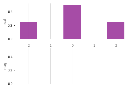
In the bar plots, real coefficients are shown in the top panel, and complex in the bottom. The labels along the x-axis represent the coefficient frequencies (for large plots, it is sometimes convenient to remove these by passing show_freqs=False to the plotting function).

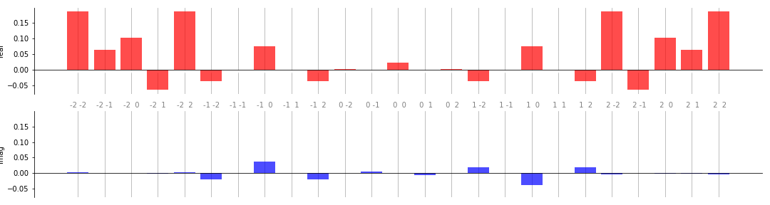
Below is a more complex example that demonstrates some of the additional customization options available:

from functools import partial

weights = np.array([[0.1, 0.2, 0.3], [0.4, 0.5, 0.6]])

@qml.qnode(dev)
def circuit_with_weights(w, x):
    qml.RX(x[0], wires=0)
    qml.RY(x[1], wires=1)
    qml.CNOT(wires=[1, 0])

    qml.Rot(*w[0], wires=0)
    qml.Rot(*w[1], wires=1)
    qml.CNOT(wires=[1, 0])

    qml.RX(x[0], wires=0)
    qml.RY(x[1], wires=1)
    qml.CNOT(wires=[1, 0])

    return qml.expval(qml.PauliZ(0))

coeffs = coefficients(partial(circuit_with_weights, weights), 2, 2)

# Number of inputs is now 2; pass custom colours as well
fig, ax = plt.subplots(2, 1, sharex=True, sharey=True, figsize=(15, 4))
bar(coeffs, 2, ax, colour_dict={"real" : "red", "imag" : "blue"})

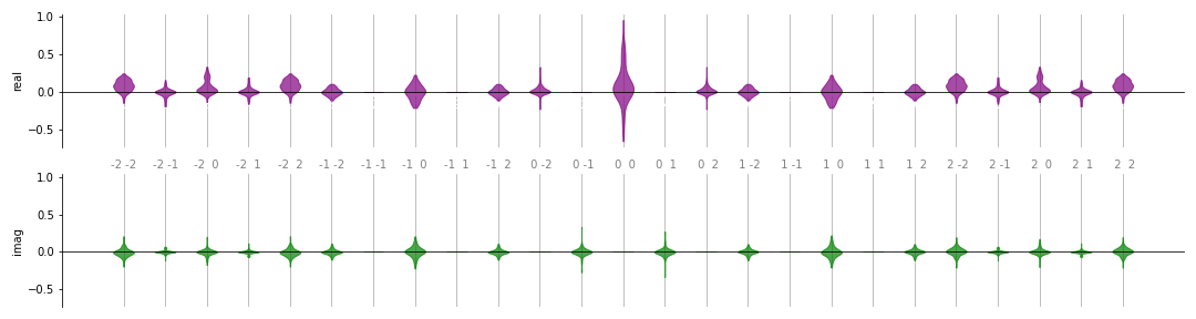
Visualizing multiple sets of coefficients

Suppose we do not want to visualize the Fourier coefficients for a fixed weights argument in circuit_with_weights, but the distribution over sets of Fourier coefficients when the weights are randomly sampled. For each weights sample we get a different set of coefficients:

coeffs = []

for _ in range(100):
    weights = np.random.normal(0, 1, size=(2, 3))
    c = coefficients(partial(circuit_with_weights, weights), 2, degree=2)
    coeffs.append(np.round(c, decimals=8))

One option to plot the distribution is violin():

fig, ax = plt.subplots(2, 1, sharey=True, figsize=(15, 4))
violin(coeffs, 2, ax, show_freqs=True)

A similar option is box(), which produces a plot of the same format but using a box plot.

A different view can obtained using the radial_box() function. This “rolls up” the coefficients onto a polar grid. Let us use it to visualize the same set of coefficients as above:

# The subplot axes must be *polar* for the radial plots
fig, ax = plt.subplots(
    1, 2, sharex=True, sharey=True,
    subplot_kw=dict(polar=True),
    figsize=(15, 8)
)
radial_box(coeffs, 2, ax, show_freqs=True, show_fliers=False)

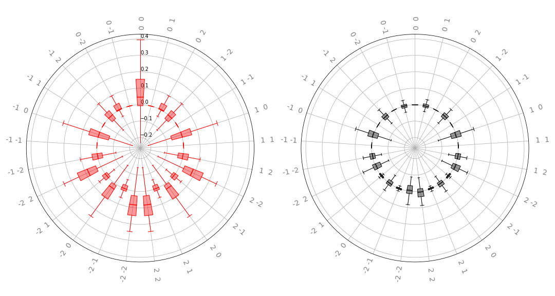
The left plot displays the real part, and the right the imaginary part of the distribution over a parametrized quantum circuit’s Fourier coefficients. The labels on the “spokes” of the wheels represent the particular frequencies; we see that this matches the coefficients we found earlier. Note how the coefficient \(c_0\) appears in the top middle of each plot; the negative frequencies extend counterclockwise from that point, and the positive frequencies increase in the clockwise direction. Such plots allow for a more compact representation of a large number of frequencies than the linear violin and box plots discussed above. For a large number of frequencies, however, it is recommended to disable the frequency labelling by setting show_freqs=False, and hiding box plot fliers as was done above.

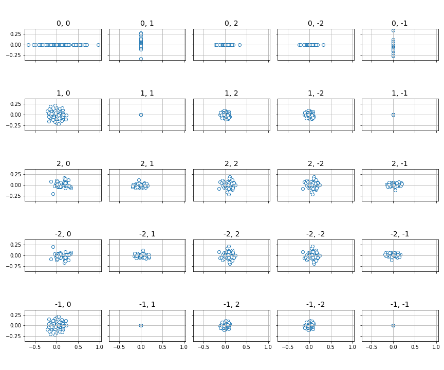
Finally, for the special case of 1- or 2-dimensional functions, we can use the panel() function to plot the distributions of the sampled sets of Fourier coefficients on the complex plane.

# Need a grid large enough to hold all coefficients up to frequency 2
fig, ax = plt.subplots(5, 5, figsize=(12, 10), sharex=True, sharey=True)
panel(coeffs, 2, ax)

code/qml_fourier

 

Download Python script

 

Download Notebook

 

View on GitHub