qml.transforms.fold_global

fold_global(tape, scale_factor)

Differentiable circuit folding of the global unitary circuit.

For a unitary circuit \(U = L_d .. L_1\), where \(L_i\) can be either a gate or layer, fold_global constructs

\[\text{fold_global}(U) = U (U^\dagger U)^n (L^\dagger_d L^\dagger_{d-1} .. L^\dagger_s) (L_s .. L_d)\]

where \(n = \lfloor (\lambda - 1)/2 \rfloor\) and \(s = \lfloor \left(\lambda - 1 \right) (d/2) \rfloor\) are determined via the scale_factor \(=\lambda\). The purpose of folding is to artificially increase the noise for zero noise extrapolation, see mitigate_with_zne().

Parameters

• tape (QNode or QuantumTape) – the quantum circuit to be folded

• scale_factor (float) – Scale factor \(\lambda\) determining \(n\) and \(s\)

Returns

The folded circuit as described in qml.transform.

Return type

qnode (QNode) or tuple[List[QuantumTape], function]

See also

mitigate_with_zne(); This function is analogous to the implementation in mitiq mitiq.zne.scaling.fold_global.

Note

This method no longer decomposes the circuit as part of the folding procedure. Users are encouraged to use decompose() to expand the circuit into a target gateset before using this transform.

Example

Let us look at the following circuit.

x = np.arange(6)

@qml.qnode(dev)
def circuit(x):
    qml.RX(x[0], wires=0)
    qml.RY(x[1], wires=1)
    qml.RZ(x[2], wires=2)
    qml.CNOT(wires=(0,1))
    qml.CNOT(wires=(1,2))
    qml.RX(x[3], wires=0)
    qml.RY(x[4], wires=1)
    qml.RZ(x[5], wires=2)
    return qml.expval(qml.Z(0) @ qml.Z(1) @ qml.Z(2))

Setting scale_factor=1 does not affect the circuit:

>>> folded = qml.transforms.fold_global(circuit, 1)
>>> print(qml.draw(folded)(x))
0: ──RX(0.0)─╭●──RX(3.0)──────────┤ ╭<Z@Z@Z>
1: ──RY(1.0)─╰X─╭●────────RY(4.0)─┤ ├<Z@Z@Z>
2: ──RZ(2.0)────╰X────────RZ(5.0)─┤ ╰<Z@Z@Z>

Setting scale_factor=2 results in the partially folded circuit \(U (L^\dagger_d L^\dagger_{d-1} .. L^\dagger_s) (L_s .. L_d)\) with \(s = \lfloor \left(1 \mod 2 \right) d/2 \rfloor = 4\) since the circuit is composed of \(d=8\) gates.

>>> folded = qml.transforms.fold_global(circuit, 2)
>>> print(qml.draw(folded)(x))
0: ──RX(0.0)─╭●──RX(3.0)──RX(3.0)†──RX(3.0)──────────────────┤ ╭<Z@Z@Z>
1: ──RY(1.0)─╰X─╭●────────RY(4.0)───RY(4.0)†─╭●──╭●──RY(4.0)─┤ ├<Z@Z@Z>
2: ──RZ(2.0)────╰X────────RZ(5.0)───RZ(5.0)†─╰X†─╰X──RZ(5.0)─┤ ╰<Z@Z@Z>

Setting scale_factor=3 results in the folded circuit \(U (U^\dagger U)\).

>>> folded = qml.transforms.fold_global(circuit, 3)
>>> print(qml.draw(folded)(x))
0: ──RX(0.0)─╭●──RX(3.0)──RX(3.0)†───────────────╭●─────────RX(0.0)†──RX(0.0)─╭●──RX(3.0)──────────┤╭<Z@Z@Z>
1: ──RY(1.0)─╰X─╭●────────RY(4.0)───RY(4.0)†─╭●──╰X†────────RY(1.0)†──RY(1.0)─╰X─╭●────────RY(4.0)─┤├<Z@Z@Z>
2: ──RZ(2.0)────╰X────────RZ(5.0)───RZ(5.0)†─╰X†──RZ(2.0)†──RZ(2.0)──────────────╰X────────RZ(5.0)─┤╰<Z@Z@Z>

Note

Circuits are treated as lists of operations. Since the ordering of that list is ambiguous, so is its folding. This can be seen exemplarily for two equivalent unitaries \(U1 = X(0) Y(0) X(1) Y(1)\) and \(U2 = X(0) X(1) Y(0) Y(1)\). The folded circuits according to scale_factor=2 would be \(U1 (X(0) Y(0) Y(0) X(0))\) and \(U2 (X(0) X(1) X(1) X(0))\), respectively. So even though \(U1\) and \(U2\) are describing the same quantum circuit, the ambiguity in their ordering as a list yields two differently folded circuits.

Usage Details

The main purpose of folding is for zero noise extrapolation (ZNE). PennyLane provides a differentiable transform mitigate_with_zne() that allows you to perform ZNE as a black box. If you want more control and see the extrapolation, you can follow the logic of the following example.

We start by setting up a noisy device using the mixed state simulator and a noise channel.

n_wires = 4

# Describe noise
noise_gate = qml.DepolarizingChannel
noise_strength = 0.05

# Load devices
dev_ideal = qml.device("default.mixed", wires=n_wires)
dev_noisy = qml.transforms.insert(noise_gate, noise_strength)(dev_ideal)

x = np.arange(6)

H = 1.*qml.X(0) @ qml.X(1) + 1.*qml.X(1) @ qml.X(2)

def circuit(x):
    qml.RY(x[0], wires=0)
    qml.RY(x[1], wires=1)
    qml.RY(x[2], wires=2)
    qml.CNOT(wires=(0,1))
    qml.CNOT(wires=(1,2))
    qml.RY(x[3], wires=0)
    qml.RY(x[4], wires=1)
    qml.RY(x[5], wires=2)
    return qml.expval(H)

qnode_ideal = qml.QNode(circuit, dev_ideal)
qnode_noisy = qml.QNode(circuit, dev_noisy)

We can then create folded versions of the noisy qnode and execute them for different scaling factors.

>>> scale_factors = [1., 2., 3.]
>>> folded_res = [qml.transforms.fold_global(qnode_noisy, lambda_)(x) for lambda_ in scale_factors]

We want to later compare the ZNE with the ideal result.

>>> ideal_res = qnode_ideal(x)

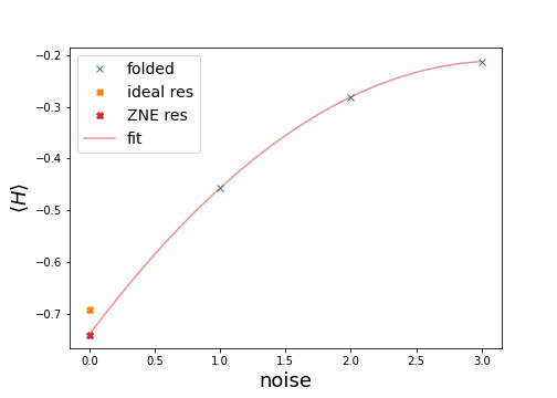
ZNE is, as the name suggests, an extrapolation in the noise to zero. The underlyding assumption is that the level of noise is proportional to the scaling factor by artificially increasing the circuit depth. We can perform a polynomial fit using numpy functions. Note that internally in mitigate_with_zne() a differentiable polynomial fit function poly_extrapolate() is used.

>>> # coefficients are ordered like coeffs[0] * x**2 + coeffs[1] * x + coeffs[0]
>>> coeffs = np.polyfit(scale_factors, folded_res, 2)
>>> zne_res = coeffs[-1]

We used a polynomial fit of order=2. Using order=len(scale_factors) -1 is also referred to as Richardson extrapolation and implemented in richardson_extrapolate(). We can now visualize our fit to see how close we get to the ideal result with this mitigation technique.

x_fit = np.linspace(0, 3, 20)
y_fit = np.poly1d(coeffs)(x_fit)

plt.plot(scale_factors, folded_res, "x--", label="folded")
plt.plot(0, ideal_res, "X", label="ideal res")
plt.plot(0, zne_res, "X", label="ZNE res", color="tab:red")
plt.plot(x_fit, y_fit, label="fit", color="tab:red", alpha=0.5)
plt.legend()

code/api/pennylane.transforms.fold_global

 

Download Python script

 

Download Notebook

 

View on GitHub