qml.qchem.molecular_hamiltonian

molecular_hamiltonian(symbols, coordinates, name='molecule', charge=0, mult=1, basis='sto-3g', method='dhf', active_electrons=None, active_orbitals=None, mapping='jordan_wigner', outpath='.', wires=None, alpha=None, coeff=None, args=None, load_data=False, convert_tol=1000000000000.0)

Generate the qubit Hamiltonian of a molecule.

This function drives the construction of the second-quantized electronic Hamiltonian of a molecule and its transformation to the basis of Pauli matrices.

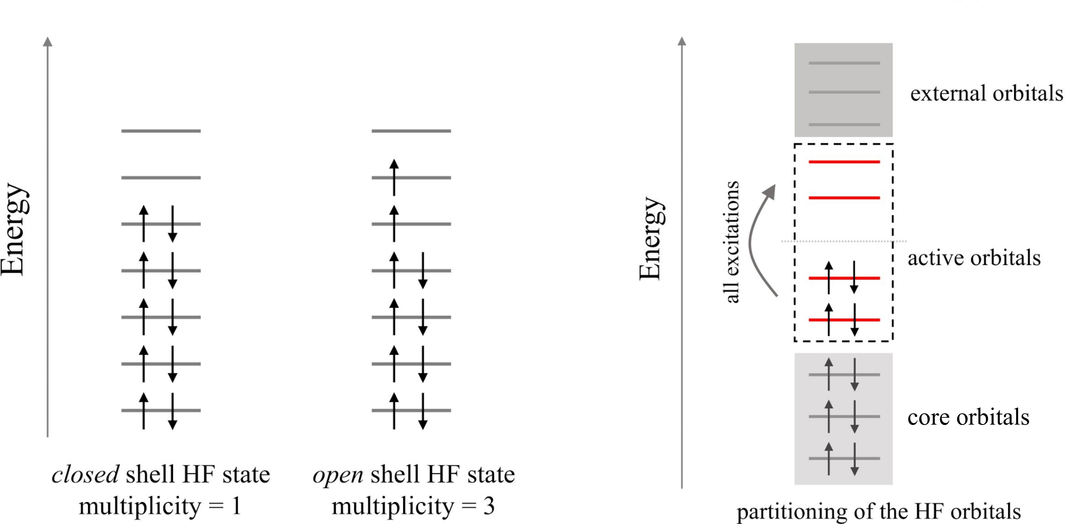
The net charge of the molecule can be given to simulate cationic/anionic systems. Also, the spin multiplicity can be input to determine the number of unpaired electrons occupying the HF orbitals as illustrated in the left panel of the figure below.

The basis of Gaussian-type atomic orbitals used to represent the molecular orbitals can be specified to go beyond the minimum basis approximation.

An active space can be defined for a given number of active electrons occupying a reduced set of active orbitals as sketched in the right panel of the figure below.

Parameters

• symbols (list[str]) – symbols of the atomic species in the molecule

• coordinates (array[float]) – atomic positions in Cartesian coordinates. The atomic coordinates must be in atomic units and can be given as either a 1D array of size 3*N, or a 2D array of shape (N, 3) where N is the number of atoms.

• name (str) – name of the molecule

• charge (int) – Net charge of the molecule. If not specified a neutral system is assumed.

• mult (int) – Spin multiplicity \(\mathrm{mult}=N_\mathrm{unpaired} + 1\) for \(N_\mathrm{unpaired}\) unpaired electrons occupying the HF orbitals. Possible values of mult are \(1, 2, 3, \ldots\). If not specified, a closed-shell HF state is assumed.

• basis (str) – atomic basis set used to represent the molecular orbitals

• method (str) – Quantum chemistry method used to solve the mean field electronic structure problem. Available options are method="dhf" to specify the built-in differentiable Hartree-Fock solver, or method="pyscf" to use the OpenFermion-PySCF plugin (this requires openfermionpyscf to be installed).

• active_electrons (int) – Number of active electrons. If not specified, all electrons are considered to be active.

• active_orbitals (int) – Number of active orbitals. If not specified, all orbitals are considered to be active.

• mapping (str) – transformation used to map the fermionic Hamiltonian to the qubit Hamiltonian

• outpath (str) – path to the directory containing output files

• wires (Wires, list, tuple, dict) – Custom wire mapping for connecting to Pennylane ansatz. For types Wires/list/tuple, each item in the iterable represents a wire label corresponding to the qubit number equal to its index. For type dict, only int-keyed dict (for qubit-to-wire conversion) is accepted for partial mapping. If None, will use identity map.

• alpha (array[float]) – exponents of the primitive Gaussian functions

• coeff (array[float]) – coefficients of the contracted Gaussian functions

• args (array[array[float]]) – initial values of the differentiable parameters

• load_data (bool) – flag to load data from the basis-set-exchange library

• convert_tol (float) – Tolerance in machine epsilon for the imaginary part of the Hamiltonian coefficients created by openfermion. Coefficients with imaginary part less than 2.22e-16*tol are considered to be real.

Returns

the fermionic-to-qubit transformed Hamiltonian and the number of qubits

Return type

tuple[pennylane.Hamiltonian, int]

Example

>>> symbols, coordinates = (['H', 'H'], np.array([0., 0., -0.66140414, 0., 0., 0.66140414]))
>>> H, qubits = molecular_hamiltonian(symbols, coordinates)
>>> print(qubits)
4
>>> print(H)
(-0.04207897647782188) [I0]
+ (0.17771287465139934) [Z0]
+ (0.1777128746513993) [Z1]
+ (-0.24274280513140484) [Z2]
+ (-0.24274280513140484) [Z3]
+ (0.17059738328801055) [Z0 Z1]
+ (0.04475014401535161) [Y0 X1 X2 Y3]
+ (-0.04475014401535161) [Y0 Y1 X2 X3]
+ (-0.04475014401535161) [X0 X1 Y2 Y3]
+ (0.04475014401535161) [X0 Y1 Y2 X3]
+ (0.12293305056183801) [Z0 Z2]
+ (0.1676831945771896) [Z0 Z3]
+ (0.1676831945771896) [Z1 Z2]
+ (0.12293305056183801) [Z1 Z3]
+ (0.176276408043196) [Z2 Z3]

code/api/pennylane.qchem.molecular_hamiltonian

 

Download Python script

 

Download Notebook

 

View on GitHub