Architectural overview
PennyLane’s core feature is the ability to compute gradients of variational quantum circuits in a way that is compatible with classical techniques such as backpropagation. PennyLane thus extends the automatic differentiation algorithms common in optimization and machine learning to include quantum and hybrid computations. A plugin system makes the framework compatible with many quantum simulators or hardware devices, remote or local.
This architectural overview introduces the basic building blocks and terminology used by PennyLane.
Components
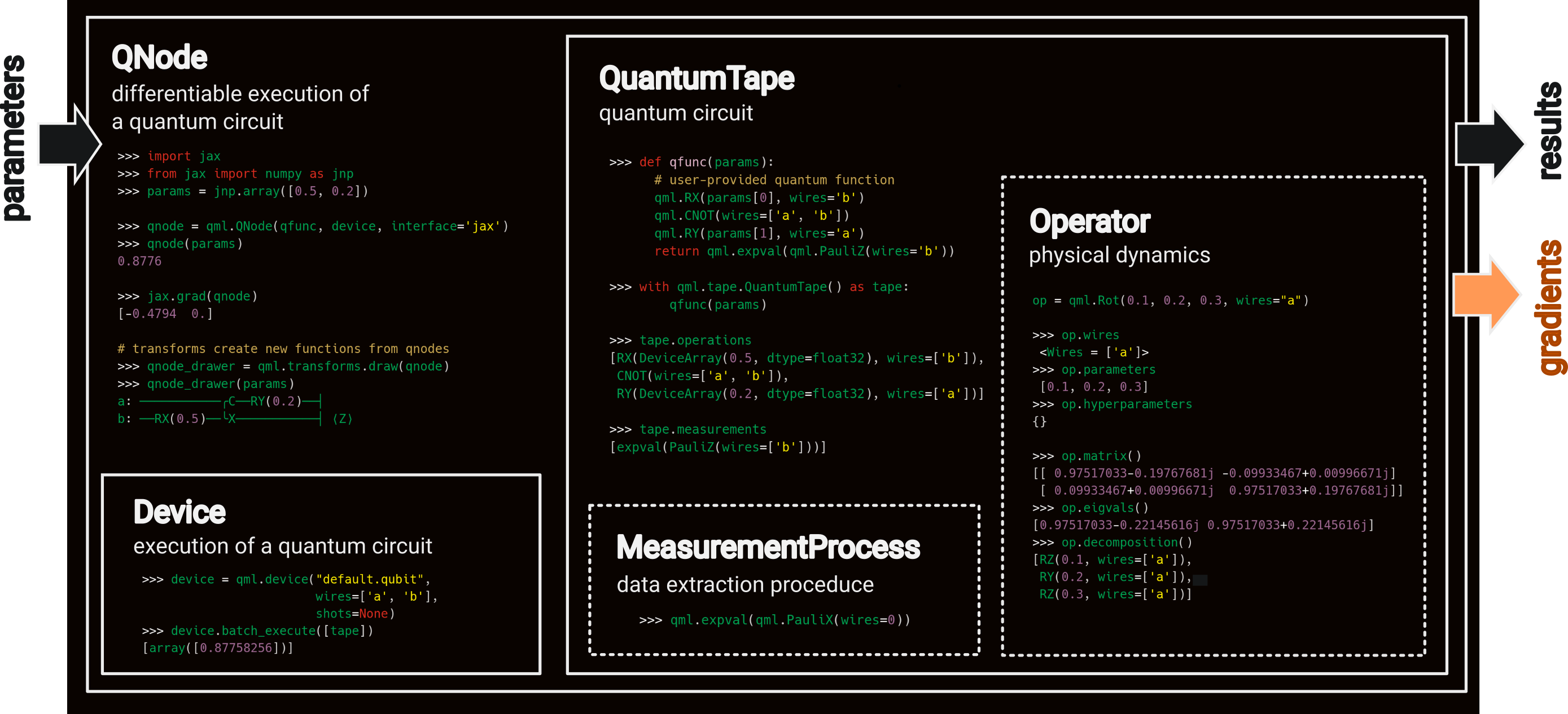
The central object in PennyLane is a QNode, which represents a “node” performing a quantum computation. Several quantum nodes may be part of a larger hybrid quantum-classical computation.
QNodes run quantum circuits on devices. The devices may be simulators built into PennyLane, or external devices provided by plugins.
The quantum circuit is specified by defining a quantum function,
which is a Python function that contains quantum operations and measurements
represented by the Operator and MeasurementProcess classes,
respectively.
Internally, the quantum function is used to construct one or more quantum tapes. A quantum tape is a context manager that records a queue of instructions required to run a quantum circuit.

The power of a QNode lies in the fact that it can be run in a “forward” fashion to execute the quantum circuit, or in a “backward” fashion in which it provides gradients (or, more precisely, jacobian-vector products).
Let’s go through these components one-by-one, this time from the “inside out” of the schematic drawing above.
Operator
Quantum operators are represented by the Operator class.
Operators are uniquely defined by their name, their (trainable) parameters, their (non-trainable) hyperparameters, and the wires they act on. Note that the trainable parameters can be tensors of any supported autodifferentiation framework.
These four defining properties are accessible for all Operator instances:
>>> from jax import numpy as jnp
>>> op = qp.Rot(jnp.array(0.1), jnp.array(0.2), jnp.array(0.3), wires=["a"])
>>> op.name
Rot
>>> op.parameters
[Array(0.1, dtype=float32, weak_type=True),
 Array(0.2, dtype=float32, weak_type=True),
 Array(0.3, dtype=float32, weak_type=True)]
>>> op.hyperparameters
{}
>>> op.wires
Wires(['a'])
Operators can optionally define the transformation they implement via symbolic or numerical representations. Here are two examples, and you find more details in the documentation on adding operations:
Representation as a product of operators
>>> op = qp.Rot(0.1, 0.2, 0.3, wires=["a"])
>>> op.decomposition()
[RZ(0.1, wires=['a']), RY(0.2, wires=['a']), RZ(0.3, wires=['a'])]
Representation as a matrix
>>> op = qp.PauliRot(0.2, "X", wires=["b"])
>>> op.matrix()
[[9.95004177e-01-2.25761781e-18j 2.72169462e-17-9.98334214e-02j]
 [2.72169462e-17-9.98334214e-02j 9.95004177e-01-2.25761781e-18j]]
Devices query operators for their properties and representations to gain information on how to implement the operator.
MeasurementProcess
While the Operator class describes a physical system and its dynamics,
the pennylane.measurement.MeasurementProcess class describes how we extract information from the quantum system.
Each measurement in pennylane has a specific class that inherits from pennylane.measurement.MeasurementProcess.
The measurement functions such as expval() create an instance of its corresponding
class (pennylane.measurements.ExpectationMP).
>>> m = qp.expval(qp.PauliZ("a"))
>>> type(m)
<class 'pennylane.measurements.expval.ExpectationMP'>
An instance of the MeasurementProcess class specifies the measured observables,
which are themselves operators.
>>> m.obs
PauliZ(wires=['a'])
For more information, check out the documentation on measurements
QuantumTape
Quantum operators and measurement processes can be used to build a quantum circuit. The user defines the circuit by constructing a quantum function, such as:
def qfunc(params):
    qp.RX(params[0], wires='b')
    qp.CNOT(wires=['a', 'b'])
    qp.RY(params[1], wires='a')
    return qp.expval(qp.PauliZ(wires='b'))
Internally, a quantum function is translated to a quantum tape, which is
the central representation of a quantum circuit. The tape is a context manager that stores lists
of Operator and MeasurementProcesses instances.
If we call the quantum function in a tape context, the
gates are stored in the tape’s operation property, while the
measurement functions such as expval() are responsible for adding measurement processes
to the tape’s measurement property.
>>> with qp.tape.QuantumTape() as tape:
...     qfunc(params)
>>> tape.operations
[RX(Array(0.5, dtype=float32), wires=['b']),
 CNOT(wires=['a', 'b']),
 RY(Array(0.2, dtype=float32), wires=['a'])]
>>> tape.measurements
[expval(PauliZ(wires=['b']))]
These two “queues” are used by devices to get information on the circuit they have to run.
Note
Tapes can represent parts of quantum circuits and do not necessarily need to define a measurement. They can also be nested.
Devices
In PennyLane, the abstraction of a quantum computation device is encompassed
within the pennylane.devices.Device class. The main job of devices is to
interpret and execute tapes. The most important method is batch_execute,
which executes a list of tapes, such as a list of the single tape created above:
>>> device = qp.device("default.qubit", wires=['a', 'b'], shots=None)
>>> device.batch_execute([tape])
[array([0.87758256])]
There are also device subclasses available, containing shared logic for
particular types of devices. For example, qubit-based devices can inherit from
the QubitDevice class, easing development.
To register a new device with PennyLane, a device subclass has to be created and registered
as an entry point under the pennylane.plugins
namespace using Setuptools. Once registered, the device can be instantiated using the device()
loader function, using the device’s name.
A Python package that registers one or more PennyLane devices is known as a plugin. For more details on plugins and devices, see Building a plugin.
QNodes
This is where it all comes together: A QNode is an encapsulation of a function \(f(x;\theta)=R^m\rightarrow R^n\) that is executed using quantum information processing on a quantum device. It is created by a quantum function and a device.
>>> import jax
>>> from jax import numpy as jnp
>>> params = jnp.array([0.5, 0.2])
>>> qnode = qp.QNode(qfunc, device, interface='jax')
>>> qnode(params)
0.8776
>>> qnode_drawer = qp.draw(qnode)
>>> print(qnode_drawer(params))
a: ───────────╭●──RY(0.20)─┤
b: ──RX(0.50)─╰X───────────┤  <Z>
Note
Users don’t typically instantiate QNodes directly—instead, the qnode() decorator or
QNode() constructor function automates the process of creating a QNode from a provided
quantum function and device.
Internally, the QNode translates the quantum function into one or more quantum tapes and classical processing routines that, taken together, execute the quantum computation.
The crucial property of a QNode is that it is differentiable by classical autodifferentiation frameworks such as autograd, JAX, and PyTorch.
>>> jax.grad(qnode)
[-0.4794  0.]
Workflow
Autodifferentiation frameworks may run QNodes in “forward mode” to compute the result of a quantum circuit, or in “backward mode” to compute the gradient of a qnode with respect to some trainable parameters.
The internal workflow in the QNode is surprisingly similar in both cases, and consists of three steps: to construct one or more tapes using the quantum function, to run the tapes on the device, and to post-process the results. The classical processing of this pipeline maintains differentiability, so that we can not only compute the result, but the gradient of the result with respect to the trainable parameters.

The fact that multiple tapes can be constructed from one quantum function may be surprising at first, but there are many situations in which the evaluation of a quantum circuit practically requires many circuits to be evaluated, for example:
When the observable is a Hamiltonian represented as a linear combination of Pauli words, the device may instruct the QNode to create one circuit for each Pauli word, and to compute their linear combination during post-processing.
When a gradient of the QNode is requested, and parameter-shift rules have to be used, the QNode constructs tapes in which parameters are shifted, and recombines the result to return a gradient.
Interfaces
The construction of tapes, as well as post-processing the results from executing tapes, are classical computations, and they are “tracked” by the autodifferentiation framework. In other words, these steps can invoke differentiable classical computations, such as:
Computing gate parameters of a compiled circuit, which are functions of the original gate parameters.
Computing linear combinations of expectations, for example when evaluating Hamiltonians term-by-term.
There are some devices where the execution of the quantum circuit is also tracked by the autodifferentiation framework. This is possible if the device is a simulator that is coded entirely in the framework’s language (such as a PyTorch quantum simulator).

Most devices, however, are blackboxes with regards to the autodifferentiation framework.
This means that when the execution on the device begins, autograd, JAX, and PyTorch
tensors need to be converted to formats that the device understands - which is in most cases
a representation as NumPy arrays. Likewise, the results of the execution have to be translated
back to differentiable tensors. These two conversions happen at what PennyLane calls the
“interface”, and you can specify this interface in the QNode with the interface keyword argument.