qml.Select¶

class Select(ops, control, work_wires=None, id=None)[source]¶

Bases: Operation

The Select operator, also known as multiplexer or multiplexed operation, applies different operations depending on the state of designated control wires.

$$Select|i\rangle \otimes |\psi\rangle = |i\rangle \otimes U_i |\psi\rangle$$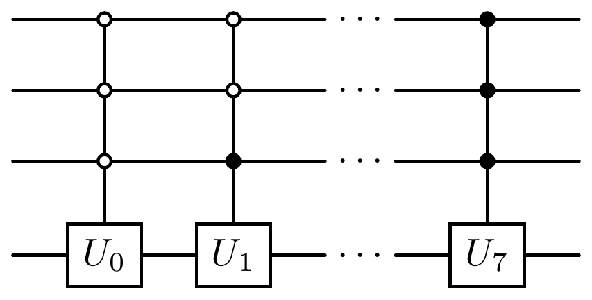

If the applied operations $\{U_i\}$ are all single-qubit Pauli rotations about the same axis, with the angle determined by the control wires, this is also called a uniformly controlled rotation gate.

See also

SelectPauliRot

Parameters:

• ops (list[Operator]) – operations to apply

• control (Sequence[int]) – the wires controlling which operation is applied. At least $\lceil \log_2 K\rceil$ wires are required for $K$ operations.

• work_wires (Union[Wires, Sequence[int], or int]) – auxiliary wire(s) that may be utilized during the decomposition of the operator into native operations. For details, see the section on the unary iterator decomposition below.

• id (str or None) – String representing the operation (optional)

Note

The position of the operation in the list determines which qubit state implements that operation. For example, when the qubit register is in the state $|00\rangle$, we will apply ops[0]. When the qubit register is in the state $|10\rangle$, we will apply ops[2]. To obtain the list position index for a given binary bitstring representing the control state we can use the following relationship: index = int(state_string, 2). For example, 2 = int('10', 2).

Example

>>> dev = qml.device('default.qubit', wires=4)
>>> ops = [qml.X(2), qml.X(3), qml.Y(2), qml.SWAP([2,3])]
>>> @qml.qnode(dev)
>>> def circuit():
>>>     qml.Select(ops, control=[0,1])
>>>     return qml.state()
...
>>> print(qml.draw(circuit, level='device')())
0: ─╭○─╭○─╭●─╭●────┤  State
1: ─├○─├●─├○─├●────┤  State
2: ─╰X─│──╰Y─├SWAP─┤  State
3: ────╰X────╰SWAP─┤  State

Unary iterator decomposition

Generically, Select is decomposed into one multi-controlled operator for each target operator. However, if auxiliary wires are available, a decomposition using a “unary iterator” can be applied. It was introduced by Babbush et al. (2018).

Principle

Unary iteration leverages auxiliary wires to store intermediate values for reuse between the different multi-controlled operators, avoiding unnecessary recomputation. In addition to this caching functionality, unary iteration reduces the cost of the computation directly, because the involved reversible AND (or Toffoli) gates can be implemented at lower cost if the target is known to be in the $|0\rangle$ state (see TemporaryAND).

For $K$ operators to be Select-applied, $c=\lceil\log_2 K\rceil$ control wires are required. Unary iteration demands an additional $c-1$ auxiliary wires. Below we first show an example for $K$ being a power of two, i.e., $K=2^c$. Then we elaborate on implementation details for the case $K<2^c$, which we call a partial Select operator.

Example

Assume that we want to Select-apply $K=8=2^3$ operators to two target wires, which requires $c=\lceil \log_2 K\rceil=3$ control wires. The generic decomposition for this takes the form

0: ─╭○─────╭○─────╭○─────╭○─────╭●─────╭●─────╭●─────╭●─────┤
1: ─├○─────├○─────├●─────├●─────├○─────├○─────├●─────├●─────┤
2: ─├○─────├●─────├○─────├●─────├○─────├●─────├○─────├●─────┤
3: ─├U(M0)─├U(M1)─├U(M2)─├U(M3)─├U(M4)─├U(M5)─├U(M6)─├U(M7)─┤
4: ─╰U(M0)─╰U(M1)─╰U(M2)─╰U(M3)─╰U(M4)─╰U(M5)─╰U(M6)─╰U(M7)─┤.

Unary iteration then uses $c-1=2$ auxiliary wires, denoted aux0 and aux1 below, to first rewrite the control structure:

0:    ─╭○───────○╮─╭○───────○╮─╭○───────○╮─╭○───────○╮─╭●───────●╮─╭●───────●╮─╭●───────●╮─╭●───────●╮─┤
1:    ─├○───────○┤─├○───────○┤─├●───────●┤─├●───────●┤─├○───────○┤─├○───────○┤─├●───────●┤─├●───────●┤─┤
aux0:  ╰─╭●───●╮─╯ ╰─╭●───●╮─╯ ╰─╭●───●╮─╯ ╰─╭●───●╮─╯ ╰─╭●───●╮─╯ ╰─╭●───●╮─╯ ╰─╭●───●╮─╯ ╰─╭●───●╮─╯ │
2:    ───├○───○┤─────├●───●┤─────├○───○┤─────├●───●┤─────├○───○┤─────├●───●┤─────├○───○┤─────├●───●┤───┤
aux1:    ╰─╭●──╯     ╰─╭●──╯     ╰─╭●──╯     ╰─╭●──╯     ╰─╭●──╯     ╰─╭●──╯     ╰─╭●──╯     ╰─╭●──╯   │
3:    ─────├U(M0)──────├U(M1)──────├U(M2)──────├U(M3)──────├U(M4)──────├U(M5)──────├U(M6)──────├U(M7)──┤
4:    ─────╰U(M0)──────╰U(M1)──────╰U(M2)──────╰U(M3)──────╰U(M4)──────╰U(M5)──────╰U(M6)──────╰U(M7)──┤

Here, we used the symbols

0: ─╭●──       ─●─╮─
1: ─├●──  and  ─●─┤─
2:  ╰───       ───╯

for TemporaryAND and its adjoint, respectively, and skipped drawing the auxiliary wires in areas where they are guaranteed to be in the state $|0\rangle$. We will need three simplification rules for pairs of TemporaryAND gates:

─○─╮─╭○──   ──     ─○─╮─╭○──   ─╭○─       ─○─╮─╭●──   ─╭●────
─○─┤─├○── = ──,    ─○─┤─├●── = ─│──, and  ─●─┤─├○── = ─│──╭●─.
───╯ ╰───   ──     ───╯ ╰───   ─╰X─       ───╯ ╰───   ─╰X─╰X─

Applying these simplifications reduces the computational cost of the Select template:

0:    ─╭○────────────────╭○──────────────────╭●─────────────────────╭●─────────────────●╮─┤
1:    ─├○────────────────│───────────────────│──╭●──────────────────│──────────────────●┤─┤
aux0:  ╰─╭●─────╭●────●╮─╰X─╭●─────╭●─────●╮─╰X─╰X─╭●─────╭●─────●╮─╰X─╭●─────╭●─────●╮─╯ │
2:    ───├○─────│─────●┤────├○─────│──────●┤───────├○─────│──────●┤────├○─────│──────●┤───┤
aux1:    ╰─╭●───╰X─╭●──╯    ╰─╭●───╰X──╭●──╯       ╰─╭●───╰X──╭●──╯    ╰─╭●───╰X──╭●──╯   │
3:    ─────├U(M0)──├U(M1)─────├U(M2)───├U(M3)────────├U(M4)───├U(M5)─────├U(M6)───├U(M7)──┤
4:    ─────╰U(M0)──╰U(M1)─────╰U(M2)───╰U(M3)────────╰U(M4)───╰U(M5)─────╰U(M6)───╰U(M7)──┤

An additional cost reduction then results from the fact that the TemporaryAND gate and its adjoint require four and zero T gates, respectively, in contrast to the seven T gates required by a decomposition of Toffoli.

For general $c$ and $K=2^c$, the decomposition takes a similar form, with alternating control and auxiliary wires.

An implementation of the unary iterator is achieved in the following steps: We first define a recursive sub-circuit R; given $L$ operators and $2 \lceil\log_2(L)\rceil + 1$ control and auxiliary wires, there are three cases that R distinguishes. First, if L>1, it applies the circuit

aux_j:   ╭R   ─╭●────╭●────●─╮─
j+1:     ├R = ─├○────│─────●─┤─
aux_j+1: ╰R    ╰──R──╰X─R────╯ ,

where each label R symbolizes a call to R itself, on the next recursion level. These next-level calls use $L' = 2^{\lceil\log_2(L)\rceil-1}$ (i.e. half of $L$, rounded up to the next power of two) and $L-L'$ (i.e. the rest) operators, respectively.

Second, if L=1, the single operator is applied, controlled on the first control wire. Finally, if L=0, R does not apply any operators.

With R defined, we are ready to outline the main circuit structure:

1. Apply the left-most TemporaryAND controlled on qubits 0 and 1.

2. Split the target operators into four “quarters” (often with varying sizes) and apply the first quarter using R.

3. Apply [X(0), CNOT([0, "aux0"]), X(0)].

4. Apply the second quarter using R.

5. Apply [CNOT([0, "aux0"]), CNOT([1, "aux0"])].

6. Apply the third quarter using R.

7. Apply [CNOT([0, "aux0"])].

8. Apply the last quarter using R.

9. Apply the right-most adjoint(TemporaryAND) controlled on qubits 0 and 1.

Partial Select decomposition

The unary iterator decomposition of the Select template can be simplified further if both of the following criteria are met:

1. There are fewer target operators than would maximally be possible for the given number of control wires, i.e. $K<2^c$.

2. The state $|\psi\rangle$ of the control wires satisfies $\langle j | \psi\rangle=0$ for all computational basis states with $j\geq K$.

We do not derive this reduction here but discuss the modifications to the implementation above that result from it.

Given $K=2^c-b$ operators, where $c$ is defined as above and we have $0\leq b<2^{c-1}$, the nine steps above are modified into one of three variants. In each variant, the first $2^{c-1}$ operators are applied in two equal portions, containing $2^{c-2}$ operators each. After this, $\ell=2^{c-1} -b$ operators remain and the three circuit variants are distinguished, based on $\ell$:

• if $\ell \geq 2^{c-2}$, the following, rather generic, circuit is applied:

  0:    ─╭○─────╭○─────╭●────────╭●─────●─╮─
  1:    ─├○─────│──────│──╭●─────│──────●─┤─
  aux0:  ╰──╭R──╰X─╭R──╰X─╰X─╭R──╰X─╭R────╯
  2:    ────├R─────├R────────├R─────├R──────
  aux1:     ╰R     ╰R        ╰R     ╰R      .
  

  Here, each operator with three R labels symbolizes a call to R. The first call in the second half applies $2^{\lceil\log_2(\ell)\rceil-1}$ operators. Note that this case is triggered if $K$ is larger than or equal to $\tfrac{3}{4}$ of the maximal capacity for $c$ control wires. Also note how the two middle TemporaryAND gates were merged into two CNOTs, like for the non-partial Select operator.

• if $1<\ell < 2^{c-2}$, the following circuit is applied:

  0:    ─╭○─────╭○─────○─╮╭●─────╭●─────●─╮─
  1:    ─├○─────│──────●─┤│──────│────────│─
  aux0:  ╰──╭R──╰X─╭R────╯│      │        │
  2:    ────├R─────├R─────├○─────│──────●─┤─
  aux1:     ╰R     ╰R     ╰───R──╰X──R────╯
  

  where the second half may skip more than one control and auxiliary wire each. In this diagram, both the operators with three and one R labels represent calls to R, with single-label instances applying fewer operators. The first call to R in the second half applies $2^{\lceil\log_2(\ell)\rceil-1}$ operators. The middle elbows act on distinct wire triples and can not be merged as above.

• if $\ell=1$, the following circuit is applied:

  0:    ─╭○─────╭○─────○─╮╭●──
  1:    ─├○─────│──────●─┤│───
  aux0:  ╰──╭R──╰X─╭R────╯│───
  2:    ────├R─────├R─────│───
  aux1:     ╰R     ╰R     ╰U  .
  

  Here, the three connected R labels symbolize a call to R and apply $2^{c-2}$ operators each. The controlled gate on the right applies the single remaining operator.

Attributes

arithmetic_depth	Arithmetic depth of the operator.
basis	The basis of an operation, or for controlled gates, of the target operation.
batch_size	Batch size of the operator if it is used with broadcasted parameters.
control	The control wires.
control_wires	Control wires of the operator.
data	Create data property
grad_method	Gradient computation method.
grad_recipe	Gradient recipe for the parameter-shift method.
has_adjoint
has_decomposition
has_diagonalizing_gates
has_generator
has_matrix
has_qfunc_decomposition
has_sparse_matrix
hash	Integer hash that uniquely represents the operator.
hyperparameters	Dictionary of non-trainable variables that this operation depends on.
id	Custom string to label a specific operator instance.
is_hermitian	This property determines if an operator is hermitian.
name	String for the name of the operator.
ndim_params	Number of dimensions per trainable parameter of the operator.
num_params	Number of trainable parameters that the operator depends on.
num_wires	Number of wires the operator acts on.
ops	Operations to be applied.
parameter_frequencies	Returns the frequencies for each operator parameter with respect to an expectation value of the form $\langle \psi | U(\mathbf{p})^\dagger \hat{O} U(\mathbf{p})|\psi\rangle$.
parameters	Trainable parameters that the operator depends on.
pauli_rep	A PauliSentence representation of the Operator, or None if it doesn't have one.
resource_keys
resource_params	A dictionary containing the minimal information needed to compute a resource estimate of the operator's decomposition.
target_wires	The wires of the target operators.
wires	All wires involved in the operation.

arithmetic_depth¶

Arithmetic depth of the operator.

basis¶

The basis of an operation, or for controlled gates, of the target operation. If not None, should take a value of "X", "Y", or "Z".

For example, X and CNOT have basis = "X", whereas ControlledPhaseShift and RZ have basis = "Z".

Type:

str or None

batch_size¶

Batch size of the operator if it is used with broadcasted parameters.

The batch_size is determined based on ndim_params and the provided parameters for the operator. If (some of) the latter have an additional dimension, and this dimension has the same size for all parameters, its size is the batch size of the operator. If no parameter has an additional dimension, the batch size is None.

Returns:

Size of the parameter broadcasting dimension if present, else None.

Return type:

int or None

control¶

The control wires.

control_wires¶

Control wires of the operator.

For operations that are not controlled, this is an empty Wires object of length 0.

Returns:

The control wires of the operation.

Return type:

Wires

data¶

Create data property

grad_method¶

Gradient computation method.

• 'A': analytic differentiation using the parameter-shift method.

• 'F': finite difference numerical differentiation.

• None: the operation may not be differentiated.

Default is 'F', or None if the Operation has zero parameters.

grad_recipe = None¶

Gradient recipe for the parameter-shift method.

This is a tuple with one nested list per operation parameter. For parameter $\phi_k$, the nested list contains elements of the form $[c_i, a_i, s_i]$ where $i$ is the index of the term, resulting in a gradient recipe of

$$\frac{\partial}{\partial\phi_k}f = \sum_{i} c_i f(a_i \phi_k + s_i).$$

If None, the default gradient recipe containing the two terms $[c_0, a_0, s_0]=[1/2, 1, \pi/2]$ and $[c_1, a_1, s_1]=[-1/2, 1, -\pi/2]$ is assumed for every parameter.

Type:

tuple(Union(list[list[float]], None)) or None

has_adjoint = False¶

has_decomposition = True¶

has_diagonalizing_gates = False¶

has_generator = False¶

has_matrix = False¶

has_qfunc_decomposition = False¶

has_sparse_matrix = False¶

hash¶

Integer hash that uniquely represents the operator.

Type:

int

hyperparameters¶

Dictionary of non-trainable variables that this operation depends on.

Type:

dict

id¶

Custom string to label a specific operator instance.

is_hermitian¶

This property determines if an operator is hermitian.

name¶

String for the name of the operator.

ndim_params¶

Number of dimensions per trainable parameter of the operator.

By default, this property returns the numbers of dimensions of the parameters used for the operator creation. If the parameter sizes for an operator subclass are fixed, this property can be overwritten to return the fixed value.

Returns:

Number of dimensions for each trainable parameter.

Return type:

tuple

num_params¶

Number of trainable parameters that the operator depends on.

By default, this property returns as many parameters as were used for the operator creation. If the number of parameters for an operator subclass is fixed, this property can be overwritten to return the fixed value.

Returns:

number of parameters

Return type:

int

num_wires = None¶

Number of wires the operator acts on.

ops¶

Operations to be applied.

parameter_frequencies¶

Returns the frequencies for each operator parameter with respect to an expectation value of the form $\langle \psi | U(\mathbf{p})^\dagger \hat{O} U(\mathbf{p})|\psi\rangle$.

These frequencies encode the behaviour of the operator $U(\mathbf{p})$ on the value of the expectation value as the parameters are modified. For more details, please see the pennylane.fourier module.

Returns:

Tuple of frequencies for each parameter. Note that only non-negative frequency values are returned.

Return type:

list[tuple[int or float]]

Example

>>> op = qml.CRot(0.4, 0.1, 0.3, wires=[0, 1])
>>> op.parameter_frequencies
[(0.5, 1), (0.5, 1), (0.5, 1)]

For operators that define a generator, the parameter frequencies are directly related to the eigenvalues of the generator:

>>> op = qml.ControlledPhaseShift(0.1, wires=[0, 1])
>>> op.parameter_frequencies
[(1,)]
>>> gen = qml.generator(op, format="observable")
>>> gen_eigvals = qml.eigvals(gen)
>>> qml.gradients.eigvals_to_frequencies(tuple(gen_eigvals))
(1.0,)

For more details on this relationship, see eigvals_to_frequencies().

parameters¶

Trainable parameters that the operator depends on.

pauli_rep¶

A PauliSentence representation of the Operator, or None if it doesn’t have one.

resource_keys = {'ops'}¶

resource_params¶

target_wires¶

The wires of the target operators.

wires¶

All wires involved in the operation.

Methods

adjoint()	Create an operation that is the adjoint of this one.
compute_decomposition(ops, control)	Representation of the operator as a product of other operators (static method).
compute_diagonalizing_gates(*params, wires, ...)	Sequence of gates that diagonalize the operator in the computational basis (static method).
compute_eigvals(*params, **hyperparams)	Eigenvalues of the operator in the computational basis (static method).
compute_matrix(*params, **hyperparams)	Representation of the operator as a canonical matrix in the computational basis (static method).
compute_qfunc_decomposition(*args, ...)	Experimental method to compute the dynamic decomposition of the operator with program capture enabled.
compute_sparse_matrix(*params[, format])	Representation of the operator as a sparse matrix in the computational basis (static method).
decomposition()	Representation of the operator as a product of other operators.
diagonalizing_gates()	Sequence of gates that diagonalize the operator in the computational basis.
eigvals()	Eigenvalues of the operator in the computational basis.
generator()	Generator of an operator that is in single-parameter-form.
label([decimals, base_label, cache])	A customizable string representation of the operator.
map_wires(wire_map)	Returns a copy of the current operator with its wires changed according to the given wire map.
matrix([wire_order])	Representation of the operator as a matrix in the computational basis.
pow(z)	A list of new operators equal to this one raised to the given power.
queue([context])	Append the operator to the Operator queue.
simplify()	Reduce the depth of nested operators to the minimum.
single_qubit_rot_angles()	The parameters required to implement a single-qubit gate as an equivalent Rot gate, up to a global phase.
sparse_matrix([wire_order, format])	Representation of the operator as a sparse matrix in the computational basis.
terms()	Representation of the operator as a linear combination of other operators.

adjoint()¶

Create an operation that is the adjoint of this one.

Adjointed operations are the conjugated and transposed version of the original operation. Adjointed ops are equivalent to the inverted operation for unitary gates.

Returns:

The adjointed operation.

static compute_decomposition(ops, control)[source]¶

Representation of the operator as a product of other operators (static method).

$$O = O_1 O_2 \dots O_n.$$

Note

Operations making up the decomposition should be queued within the compute_decomposition method.

See also

decomposition().

Parameters:

• ops (list[Operator]) – operations to apply

• control (Sequence[int]) – the wires controlling which operation is applied

Returns:

decomposition of the operator

Return type:

list[Operator]

Example

>>> ops = [qml.X(2), qml.X(3), qml.Y(2), qml.SWAP([2,3])]
>>> qml.Select.compute_decomposition(ops, control=[0,1])
[MultiControlledX(wires=[0, 1, 2], control_values=[0, 0]),
 MultiControlledX(wires=[0, 1, 3], control_values=[0, 1),
 Controlled(Y(2), control_wires=[0, 1], control_values=[True, False]),
 Controlled(SWAP(wires=[2, 3]), control_wires=[0, 1])]

static compute_diagonalizing_gates(*params, wires, **hyperparams)¶

Sequence of gates that diagonalize the operator in the computational basis (static method).

Given the eigendecomposition $O = U \Sigma U^{\dagger}$ where $\Sigma$ is a diagonal matrix containing the eigenvalues, the sequence of diagonalizing gates implements the unitary $U^{\dagger}$.

The diagonalizing gates rotate the state into the eigenbasis of the operator.

See also

diagonalizing_gates().

Parameters:

• params (list) – trainable parameters of the operator, as stored in the parameters attribute

• wires (Iterable[Any], Wires) – wires that the operator acts on

• hyperparams (dict) – non-trainable hyperparameters of the operator, as stored in the hyperparameters attribute

Returns:

list of diagonalizing gates

Return type:

list[.Operator]

static compute_eigvals(*params, **hyperparams)¶

Eigenvalues of the operator in the computational basis (static method).

If diagonalizing_gates are specified and implement a unitary $U^{\dagger}$, the operator can be reconstructed as

$$O = U \Sigma U^{\dagger},$$

where $\Sigma$ is the diagonal matrix containing the eigenvalues.

Otherwise, no particular order for the eigenvalues is guaranteed.

See also

Operator.eigvals() and qml.eigvals()

Parameters:

• *params (list) – trainable parameters of the operator, as stored in the parameters attribute

• **hyperparams (dict) – non-trainable hyperparameters of the operator, as stored in the hyperparameters attribute

Returns:

eigenvalues

Return type:

tensor_like

static compute_matrix(*params, **hyperparams)¶

Representation of the operator as a canonical matrix in the computational basis (static method).

The canonical matrix is the textbook matrix representation that does not consider wires. Implicitly, this assumes that the wires of the operator correspond to the global wire order.

See also

Operator.matrix() and qml.matrix()

Parameters:

• *params (list) – trainable parameters of the operator, as stored in the parameters attribute

• **hyperparams (dict) – non-trainable hyperparameters of the operator, as stored in the hyperparameters attribute

Returns:

matrix representation

Return type:

tensor_like

static compute_qfunc_decomposition(*args, **hyperparameters)¶

Experimental method to compute the dynamic decomposition of the operator with program capture enabled.

When the program capture feature is enabled with qml.capture.enable(), the decomposition of the operator is computed with this method if it is defined. Otherwise, the compute_decomposition() method is used.

The exception to this rule is when the operator is returned from the compute_decomposition() method of another operator, in which case the decomposition is performed with compute_decomposition() (even if this method is defined), and not with this method.

When compute_qfunc_decomposition is defined for an operator, the control flow operations within the method (specifying the decomposition of the operator) are recorded in the JAX representation.

Note

This method is experimental and subject to change.

See also

compute_decomposition().

Parameters:

• *args (list) – positional arguments passed to the operator, including trainable parameters and wires

• **hyperparameters (dict) – non-trainable hyperparameters of the operator, as stored in the hyperparameters attribute

static compute_sparse_matrix(*params, format='csr', **hyperparams)¶

Representation of the operator as a sparse matrix in the computational basis (static method).

The canonical matrix is the textbook matrix representation that does not consider wires. Implicitly, this assumes that the wires of the operator correspond to the global wire order.

See also

sparse_matrix()

Parameters:

• *params (list) – trainable parameters of the operator, as stored in the parameters attribute

• format (str) – format of the returned scipy sparse matrix, for example ‘csr’

• **hyperparams (dict) – non-trainable hyperparameters of the operator, as stored in the hyperparameters attribute

Returns:

sparse matrix representation

Return type:

scipy.sparse._csr.csr_matrix

decomposition()[source]¶

Representation of the operator as a product of other operators.

$$O = O_1 O_2 \dots O_n$$

A DecompositionUndefinedError is raised if no representation by decomposition is defined.

See also

compute_decomposition().

Returns:

decomposition of the operator

Return type:

list[Operator]

Example

>>> ops = [qml.X(2), qml.X(3), qml.Y(2), qml.SWAP([2,3])]
>>> op = qml.Select(ops, control=[0,1])
>>> op.decomposition()
[MultiControlledX(wires=[0, 1, 2], control_values=[0, 0]),
 MultiControlledX(wires=[0, 1, 3], control_values=[0, 1]),
 Controlled(Y(2), control_wires=[0, 1], control_values=[True, False]),
 Controlled(SWAP(wires=[2, 3]), control_wires=[0, 1])]

diagonalizing_gates()¶

Sequence of gates that diagonalize the operator in the computational basis.

Given the eigendecomposition $O = U \Sigma U^{\dagger}$ where $\Sigma$ is a diagonal matrix containing the eigenvalues, the sequence of diagonalizing gates implements the unitary $U^{\dagger}$.

The diagonalizing gates rotate the state into the eigenbasis of the operator.

A DiagGatesUndefinedError is raised if no representation by decomposition is defined.

See also

compute_diagonalizing_gates().

Returns:

a list of operators

Return type:

list[.Operator] or None

eigvals()¶

Eigenvalues of the operator in the computational basis.

If diagonalizing_gates are specified and implement a unitary $U^{\dagger}$, the operator can be reconstructed as

$$O = U \Sigma U^{\dagger},$$

where $\Sigma$ is the diagonal matrix containing the eigenvalues.

Otherwise, no particular order for the eigenvalues is guaranteed.

Note

When eigenvalues are not explicitly defined, they are computed automatically from the matrix representation. Currently, this computation is not differentiable.

A EigvalsUndefinedError is raised if the eigenvalues have not been defined and cannot be inferred from the matrix representation.

See also

compute_eigvals()

Returns:

eigenvalues

Return type:

tensor_like

generator()¶

Generator of an operator that is in single-parameter-form.

For example, for operator

$$U(\phi) = e^{i\phi (0.5 Y + Z\otimes X)}$$

we get the generator

>>> U.generator()
0.5 * Y(0) + Z(0) @ X(1)

The generator may also be provided in the form of a dense or sparse Hamiltonian (using LinearCombination and SparseHamiltonian respectively).

label(decimals=None, base_label=None, cache=None)¶

A customizable string representation of the operator.

Parameters:

• decimals=None (int) – If None, no parameters are included. Else, specifies how to round the parameters.

• base_label=None (str) – overwrite the non-parameter component of the label

• cache=None (dict) – dictionary that carries information between label calls in the same drawing

Returns:

label to use in drawings

Return type:

str

Example:

>>> op = qml.RX(1.23456, wires=0)
>>> op.label()
"RX"
>>> op.label(base_label="my_label")
"my_label"
>>> op = qml.RX(1.23456, wires=0, id="test_data")
>>> op.label()
"RX("test_data")"
>>> op.label(decimals=2)
"RX\n(1.23,"test_data")"
>>> op.label(base_label="my_label")
"my_label("test_data")"
>>> op.label(decimals=2, base_label="my_label")
"my_label\n(1.23,"test_data")"

If the operation has a matrix-valued parameter and a cache dictionary is provided, unique matrices will be cached in the 'matrices' key list. The label will contain the index of the matrix in the 'matrices' list.

>>> op2 = qml.QubitUnitary(np.eye(2), wires=0)
>>> cache = {'matrices': []}
>>> op2.label(cache=cache)
'U(M0)'
>>> cache['matrices']
[tensor([[1., 0.],
 [0., 1.]], requires_grad=True)]
>>> op3 = qml.QubitUnitary(np.eye(4), wires=(0,1))
>>> op3.label(cache=cache)
'U(M1)'
>>> cache['matrices']
[tensor([[1., 0.],
        [0., 1.]], requires_grad=True),
tensor([[1., 0., 0., 0.],
        [0., 1., 0., 0.],
        [0., 0., 1., 0.],
        [0., 0., 0., 1.]], requires_grad=True)]

map_wires(wire_map)[source]¶

Returns a copy of the current operator with its wires changed according to the given wire map.

Parameters:

wire_map (dict) – dictionary containing the old wires as keys and the new wires as values

Returns:

new operator

Return type:

.Operator

matrix(wire_order=None)¶

Representation of the operator as a matrix in the computational basis.

If wire_order is provided, the numerical representation considers the position of the operator’s wires in the global wire order. Otherwise, the wire order defaults to the operator’s wires.

If the matrix depends on trainable parameters, the result will be cast in the same autodifferentiation framework as the parameters.

A MatrixUndefinedError is raised if the matrix representation has not been defined.

See also

compute_matrix()

Parameters:

wire_order (Iterable) – global wire order, must contain all wire labels from the operator’s wires

Returns:

matrix representation

Return type:

tensor_like

pow(z)¶

A list of new operators equal to this one raised to the given power.

Parameters:

z (float) – exponent for the operator

Returns:

list[Operator]

queue(context=<class 'pennylane.queuing.QueuingManager'>)¶

Append the operator to the Operator queue.

simplify()¶

Reduce the depth of nested operators to the minimum.

Returns:

simplified operator

Return type:

.Operator

single_qubit_rot_angles()¶

The parameters required to implement a single-qubit gate as an equivalent Rot gate, up to a global phase.

Returns:

A list of values $[\phi, \theta, \omega]$ such that $RZ(\omega) RY(\theta) RZ(\phi)$ is equivalent to the original operation.

Return type:

tuple[float, float, float]

sparse_matrix(wire_order=None, format='csr')¶

Representation of the operator as a sparse matrix in the computational basis.

If wire_order is provided, the numerical representation considers the position of the operator’s wires in the global wire order. Otherwise, the wire order defaults to the operator’s wires.

A SparseMatrixUndefinedError is raised if the sparse matrix representation has not been defined.

See also

compute_sparse_matrix()

Parameters:

• wire_order (Iterable) – global wire order, must contain all wire labels from the operator’s wires

• format (str) – format of the returned scipy sparse matrix, for example ‘csr’

Returns:

sparse matrix representation

Return type:

scipy.sparse._csr.csr_matrix

terms()¶

Representation of the operator as a linear combination of other operators.

$$O = \sum_i c_i O_i$$

A TermsUndefinedError is raised if no representation by terms is defined.

Returns:

list of coefficients $c_i$ and list of operations $O_i$

Return type:

tuple[list[tensor_like or float], list[.Operation]]